Coordination number analysis
This analysis calculates the coordination number by simply counting the neighbors. The result is identical to the RDF integral in an isotropic system.
3D coordination number
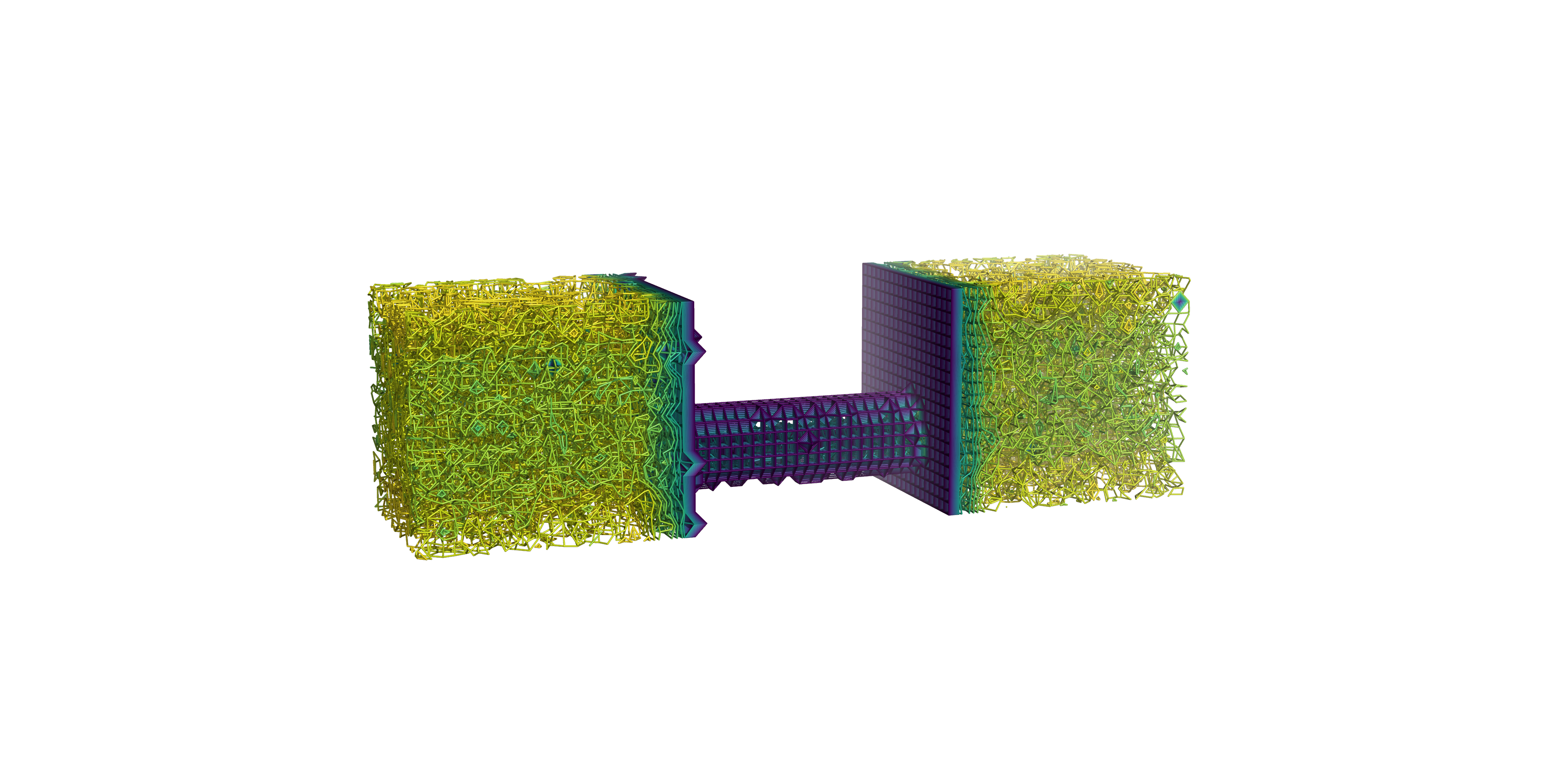
The result of the analysis can be performed on a user-defined grid and printed as a Gaussian cube file. Each 3D-bin will contain the coordination number up to the specified coordination distance. The output is split into separate cube files for each pair of species (excluding species identified or defined as structures). The cube files can be visualized to obtain a 3D map of the coordination number (using e.g. VMD, PyMol, etc.). This can be helpful to identify regions of interest in highly anisotropic systems:
Distance-dependence to structures
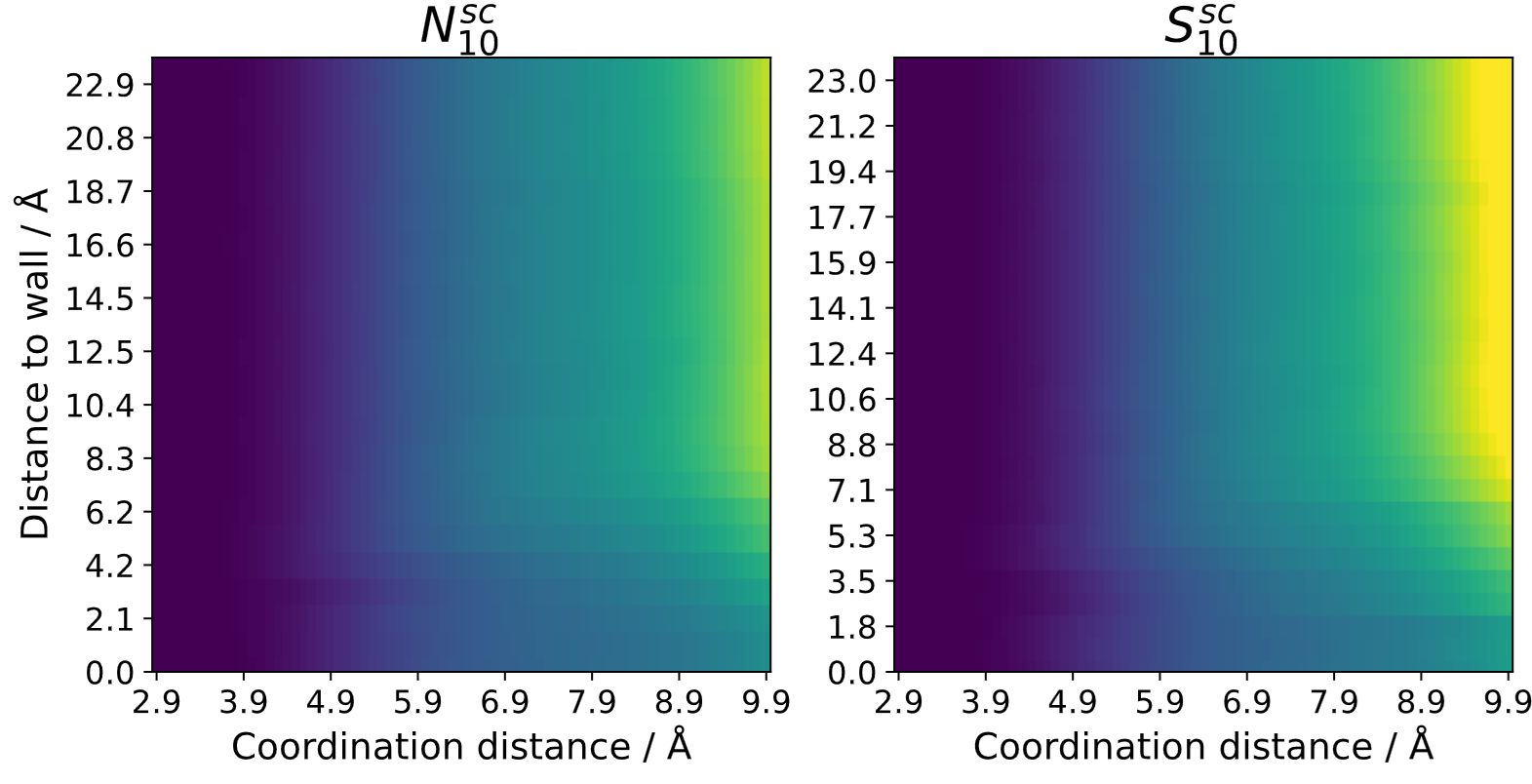
If no 3D-analysis is conducted, the coordination number can be calculated relative to structures. For any kind of structure, a 2D-heatmap can be generated where one axis contains the coordination distance and the other axis contains the distance to a reference structure. This can be utilized to see trends in transition regions going from surfaces to bulk liquid. Here is an example comparing a neat ionic liquid at a carbon surface to a system with added salt [1]:
If the system contains a porous material (e.g. nanopore) the coordination number can also be calculated inside of the pores relative to the inner pore walls:
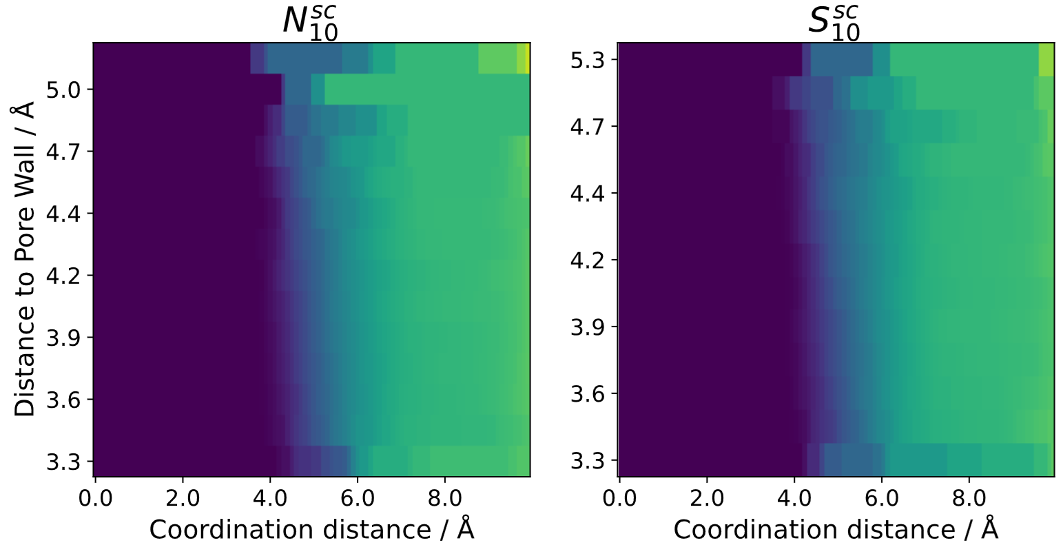
Note that this either needs really large pores or long simulation times to yield sufficient sampling, as there are usually not many atoms present inside of nanopores when compares to bulk liquid.
Note
example pictures taken from ref [1] [1].